Constant vs. nighttime-reduced temperature

asked 2016-02-04 08:11:26 -0500

nico

51 ●5

updated 2020-03-08 11:27:20 -0500

__AmirRoth__

4436 ●5 ●17 http://bleedinggreenna...

Hello,

As a new Open Studio user, I conducted a bunch of simulations to understand the impact of different parameters. Among these simulations, a case bothers me.

(Sorry, but as a new user I cannot post pictures... I had to insert links to files)

The basic version consists of a simple cube (no windows, no internal gains, no infiltration, no ventilation ...). The temperature is set to 22 °C (constant) and I make use of the "ideal air loads system". The results seem consistent (see green values in the file, which are also found in the graph)

Results without nighttime-reduced temperature

Graphic

The second version is identical but incorporating a temperature reduction at night and on weekends (16°C instead of 22°C). Of course I understand that some heating-up capacity is necessary, but this does not explain all the results.

Results with nighttime-reduced temperature

Graphic

"calculated design load" is identical in both cases, which makes sense
in the basic version, "district heating" is 3137.46W and corresponds to the peak on the graph : OK
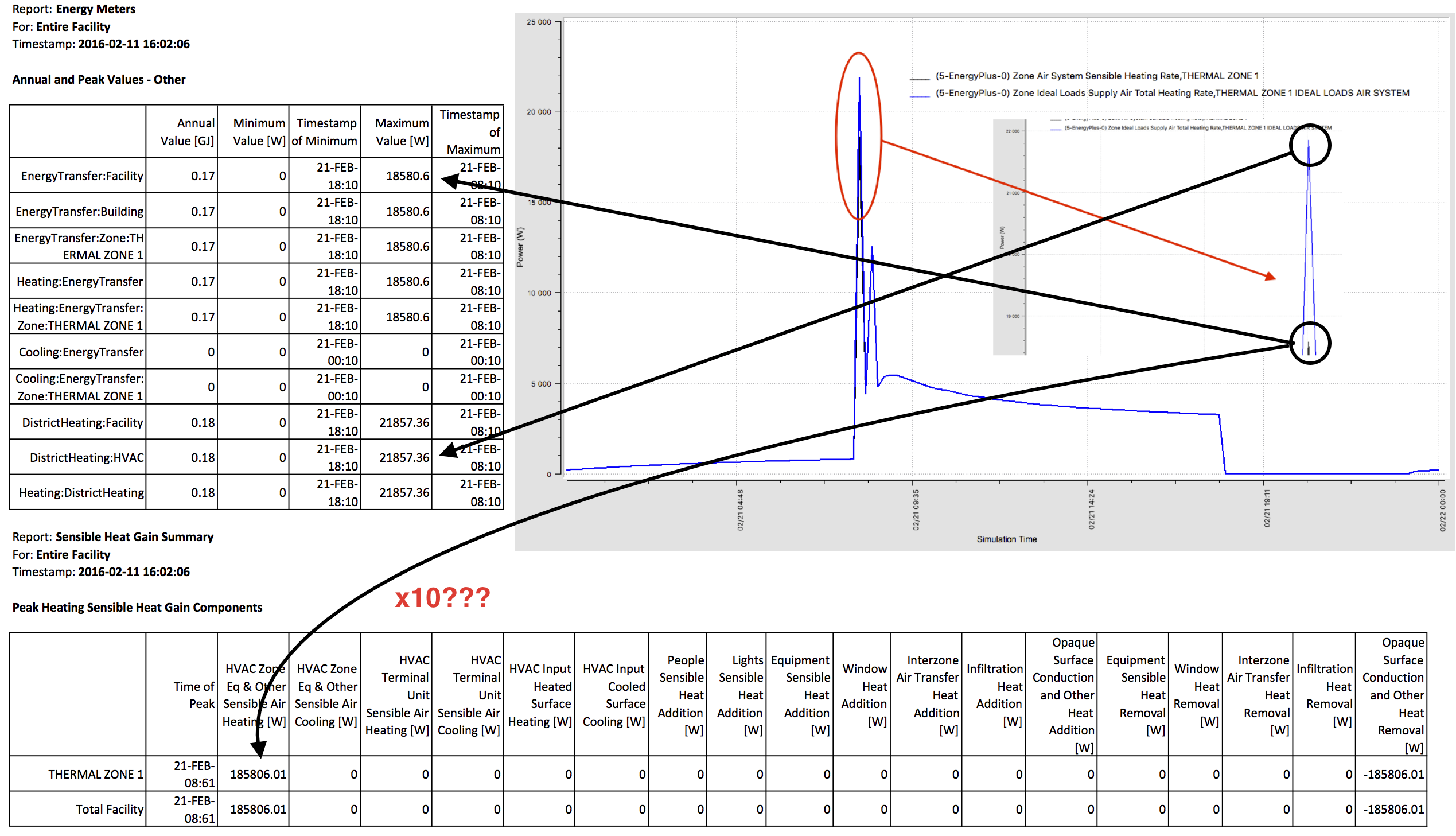
in the modified version, "district heating" is 23513.39W (almost 8 x higher). This value does not match the peak on the graph (about 9750 W). Is there an explanation?
in "energy meters", why is "Energy Transfer Partners: Facility" (20183.82 W) slightly different than "DistrictHeating:Facility" (23513.39 W) ?
where does "HVAC area eq. & Other sensitive air heating" value (188925.97 W) come from ?

Could you help me? Am I missing something?

I understand that this is an "extreme" case, and that in reality the differences will be smaller thanks to internal and solar gains (I tried a real case, and there is an order of magnitude of +/- 2).

Without modeling a complete HVAC system, is there a way to get closer to a real heating system (with limited capacity)?

Thank you very much for your time.

Nicolas

EDIT

From what I could see, the use of "Timesteps in Averaging Window" only affects the "design load" value in the report. This will certainly help me in other situations, but in fact, my question is not really about sizing (I used constant temperature set point) but the complete runperiod.

I could finally find some values by performing the simulation on a day (thank you for the tip), but there are certain factors that I can not explain :

image description

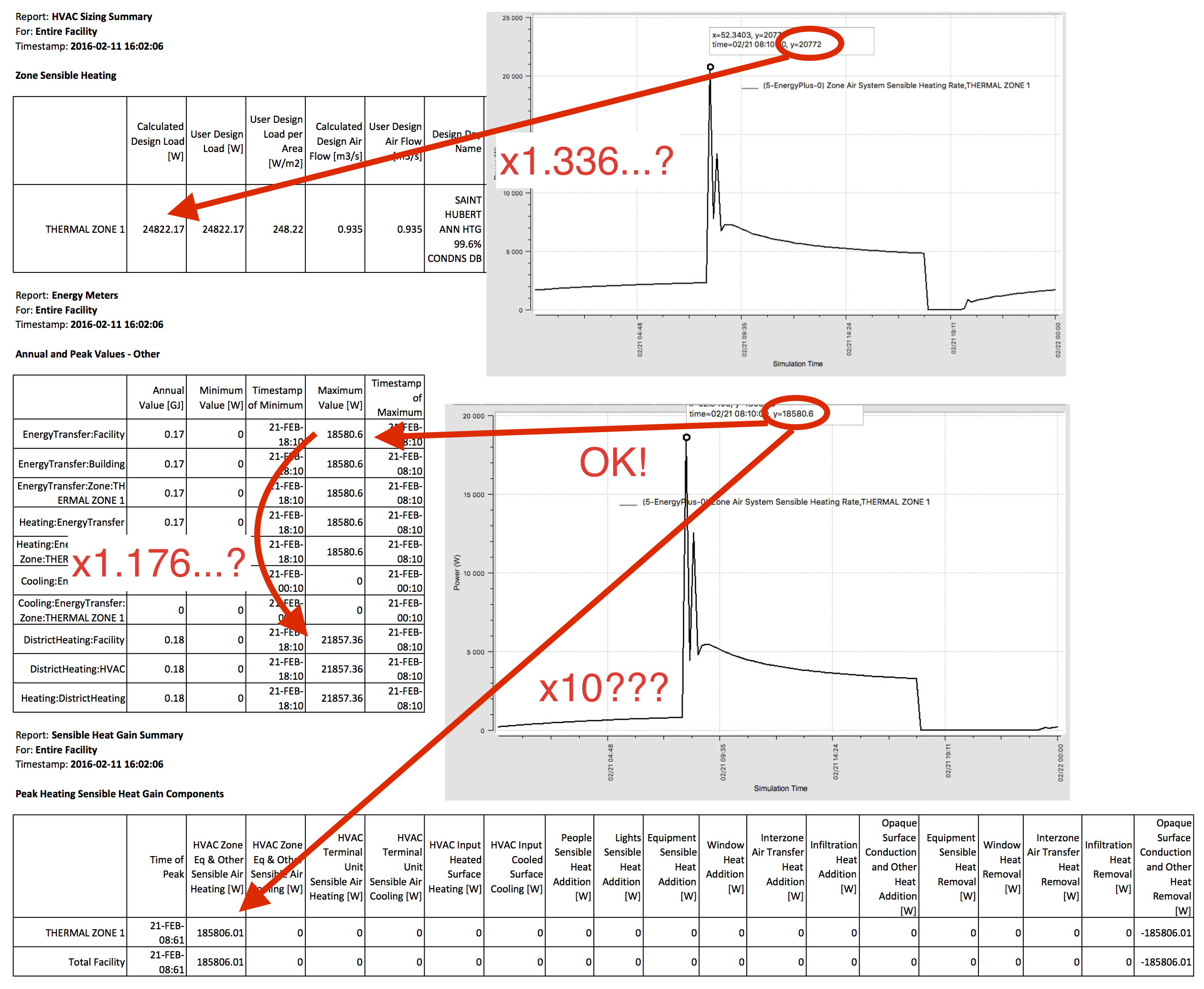
1.176 coefficient between "EnergyTransfer:Facility" and "DistrictHeating:Facility"
1.336 coefficient between the peak on the graph and the "design load" value
10 coefficient between the peak on the graph and the "peak heating sensible heat gain" value

If I use a constant schedule, these three factors are exactly 1 ...

Currently, I use "ideal loads air system". I would have to take the time to create a measure which limits the power to the "design load" value calculated in a previous run...

Here is a link to the idf file if it can help you :

IDF file

Thanks

edit retag flag offensive close merge delete

Comments

Your using zone multipliers in your simulation. Some results are not multiplied, others are.

rraustad ( 2016-02-11 11:04:21 -0500 )edit

I'd have to look at the input file to answer the other questions, but I assume 1) the conditions are not the same between the calculation of design load and the operating capacity of 20772, and 2) that EnergyTransfer:Facility includes more than DistrictHeating (check the mdd file).

rraustad ( 2016-02-11 11:33:45 -0500 )edit

add a comment

5

answered 2016-02-10 20:45:17 -0500

rraustad

13599 ●72 ●12 http://www.fsec.ucf.edu/

updated 2016-02-10 20:48:46 -0500

The use of setback/setup in the thermostat temperature schedules causes zone sizing to overestimate the load during the setup time step. For example, as the heating set point temperature changes from 16C to 22C, the load prediction becomes very large. The prediction calculates the capacity needed to bring the zone temperature all the way up to the new temperature set point.

If you are autosizing, you can either use constant temperature set points during sizing on design days, or use an averaging approach to smooth the sizing results using the Timesteps in Averaging Window input in the Sizing:Parameters object:

Timestep,4;

Sizing:Parameters,
  1.3,                     !- Heating Sizing Factor
  1.3,                     !- Cooling Sizing Factor
  8;                        !- Timesteps in Averaging Window

If you are not autosizing, this result may be due to unlimited capacity. For example, in the ZoneHVAC:IdealLoadsAirSystem.

From your graphs, I cannot tell what happens after the setup time step. There may be a spike in capacity (power) during the setup time step, but shortly after that time, certainly near the setback time step, the capacity (power) for each simulation should be very near. Try isolating a single day and view the same graphic over a shorter period of time.

Check the input for heating limit in the ideal loads air system object.

ZoneHVAC:IdealLoadsAirSystem,
  A5 , \field Heating Limit
     \type choice
     \key NoLimit
     \key LimitFlowRate
     \key LimitCapacity
     \key LimitFlowRateAndCapacity
     \default NoLimit
  N6 , \field Maximum Sensible Heating Capacity

edit flag offensive delete link

Comments

Thank you for your help! The place is missing to comment your answer, so I have edited my question.

nico ( 2016-02-11 09:58:48 -0500 )edit

add a comment

1

answered 2016-02-12 10:06:04 -0500

nico

51 ●5

OK, I am progressing :-)

Looking at the MTD file, I found that "EnergyTransfer:Facility" is based on "Zone Air System Sensible Heating Rate", while "DistrictHeating: Facility" is based on "Zone Ideal Loads Supply Air Total Heating Rate".

image description

By zooming in on the chart, we see that only the peak is different. The rest of the curve is exactly the same! If I use a constant temperature setpoint, the curves are perfectly superimposed

I still can not understand the x10 factor on "Peak Sensible Heat Gain". The model contains a single area, without multiplication factor. All coefficients worth 1.0

This x10 factor also vanishes if I use a constant temperature setpoint...

edit flag offensive delete link

Comments

What is specified for the heating limit in your input file?

ZoneHVAC:IdealLoadsAirSystem,
  A5 , \field Heating Limit

rraustad ( 2016-02-12 10:50:07 -0500 )edit

It is : NoLimit.

nico ( 2016-02-12 14:04:25 -0500 )edit

Change it to heating capacity and enter 21857.36 in the heating capacity field.

rraustad ( 2016-02-12 14:43:14 -0500 )edit

add a comment

Constant vs. nighttime-reduced temperature

Comments

2 Answers

Comments

Comments

Your Answer

Careers

Question Tools

Stats

Constant vs. nighttime-reduced temperature edit

Comments

2 Answers

Comments

Comments

Your Answer

Careers

Question Tools

Stats

Constant vs. nighttime-reduced temperature