As the name implies, I'm trying to understand what's the rationale behind the default curve that come with the chiller
Let's take for example a Chiller:Electric:EIR and look specifically are the EIRFPLR curve, that is the Electric Input Ratio as a function of the Part Load Ratio.
This curve is quadratic: $$EIR = a + b\times PLR + c \times PLR^2$$
OpenStudio has the following default coefficients: - $a = 0.06369119$, - $b = 0.58488832$ - $c = 0.35280274$.
It seems that it leads to a VERY efficient chiller, unless I'm missing something. I've compared it t:
the Comnet modeling guidelines here (Table 6.8.2-9: "Default Efficiency EIR-FPLR Coefficients – Water-Cooled Chillers" > Centrifugal)
DOE-2 Centrifugal/5.50COP from the E+ dataset (EnergyPlusV8-3-0\DataSets\Chillers.idf)
Curve fitting coefficients, based on manufacturer data for a McQuay chiller with magnetic bearings (supposed to be top of the line)
| a | b | c | |
|---|---|---|---|
| Comnet | 0.171493 | 0.588202 | 0.237373 |
| DOE-2 Centrifugal COP 5.50 | 0.222903 | 0.313387 | 0.463710 |
| McQuay | 0.164871 | 0.606613 | 0.229741 |
| OpenStudio | 0.063691 | 0.584888 | 0.352803 |
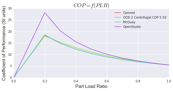
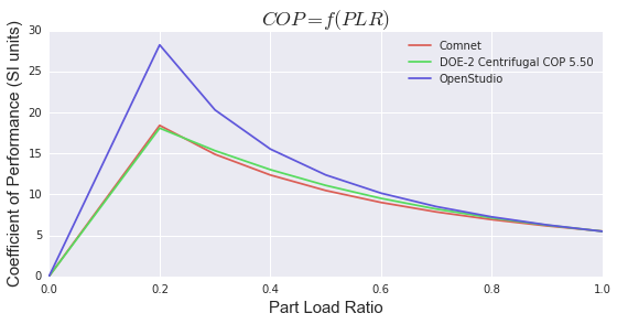
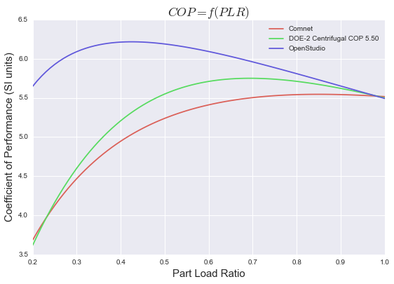
I end up with the following curves where I'm displaying COP (SI units) instead of EIR since it's more intuitive in my opinion.
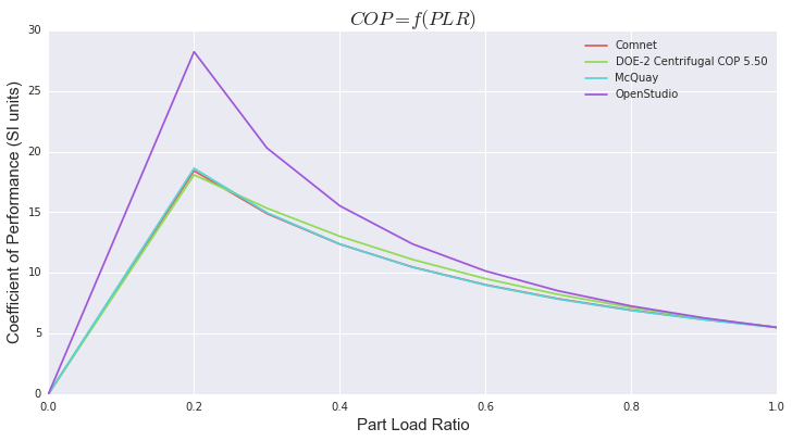
Anyone can explain why it seems so much more efficient than the rest?