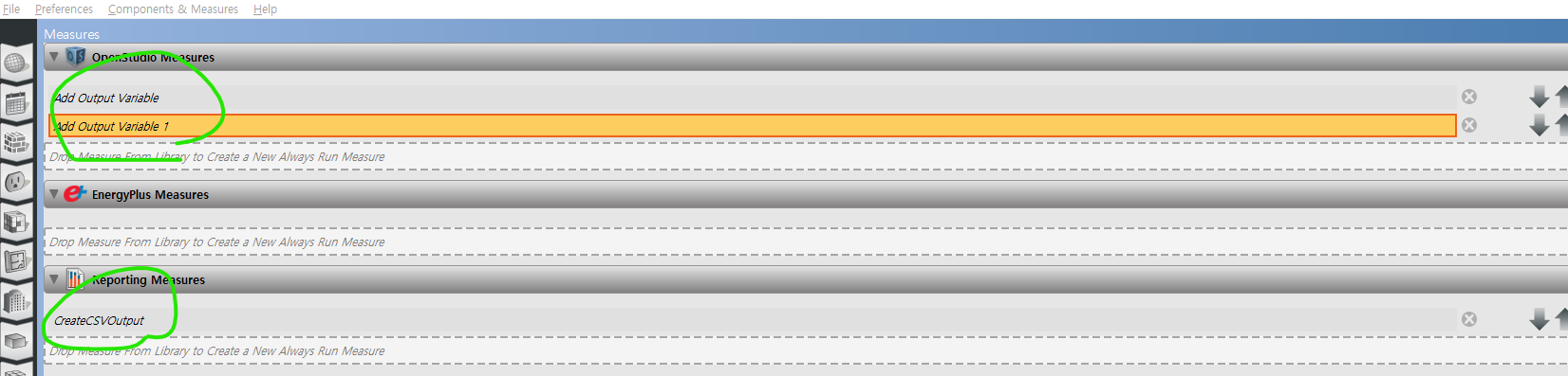
Hi Jack. I use the measure "CreateCSVOutput" in the BLC library to get a .csv file which is placed in the run folder after every simulationrun with all the variable data output. Then I use a python script to graph the data in my webbrowser.
Use ChatGPT or Google AIstudio to edit the script to your liking. I hope this helps you somewhat. Good luck.
import pandas as pd import
plotly.graph_objs as go import
plotly.io as pio import tempfile
import webbrowser import os
csv_file =
'report_variables_ZoneTimestep.csv'
df = pd.read_csv(csv_file,
parse_dates=['Zone Timestep'],
index_col='Zone Timestep')
exclude_cols = [
'e:Electricity:Facility[J]' ]
def is_power_variable(col_name: str)
-> bool:
keywords = ['[w]', '(w)', ' watt', 'power', 'rate', 'elec']
return any(k.lower() in col_name.lower() for k in keywords)
available_cols = [c for c in
df.columns if c not in exclude_cols]
left_cols = [c for c in available_cols
if not is_power_variable(c)]
right_cols = [c for c in
available_cols if
is_power_variable(c)]
fig = go.Figure()
for col in left_cols:
fig.add_trace(go.Scatter(x=df.index,
y=df[col], mode='lines', name=col,
yaxis='y1'))
for col in right_cols:
fig.add_trace(go.Scatter(x=df.index,
y=df[col], mode='lines', name=col,
yaxis='y2'))
fig.update_layout(
title='All Variables from CSV',
xaxis_title='Time',
yaxis=dict(
title='Temperature [Celsius]',
side='left',
showgrid=False,
autorange=True
),
yaxis2=dict(
title='Power [Watt]',
overlaying='y',
side='right',
showgrid=False,
autorange=True
),
hovermode='x unified',
xaxis=dict(
rangeselector=dict(
buttons=list([
dict(count=1, label='1 day', step='day',
stepmode='backward'),
dict(count=7, label='1 week', step='day',
stepmode='backward'),
dict(count=1, label='1 month', step='month',
stepmode='backward'),
dict(step='all')
])
),
rangeslider=dict(visible=True),
type='date'
) )
with tempfile.NamedTemporaryFile('w',
delete=False, suffix='.html',
encoding='utf-8') as f:
html_str = pio.to_html(fig, include_plotlyjs='cdn',
full_html=True, config={'displaylogo':
False})
f.write(html_str)
temp_path = f.name
webbrowser.open('file://' +
os.path.realpath(temp_path))
print("Base plot opened in browser.
Axis scaling now uses default Plotly
autorange.")


In this thread, a method using eso files and the postprocess
ReadVarsESO.exewas introduced. Is this the standard way? link