Revision history [back]

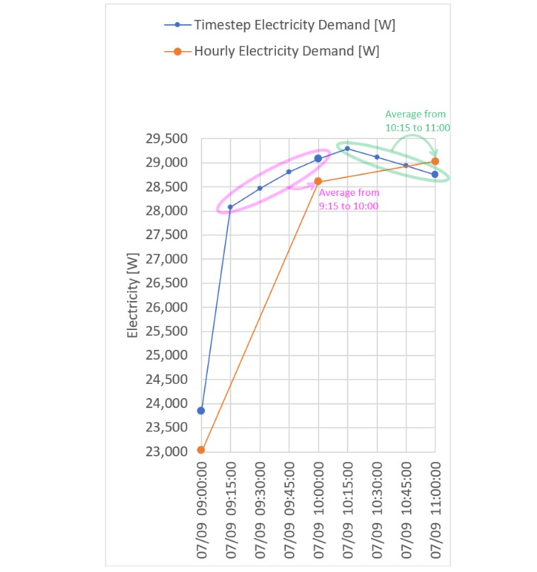
@rraustad 's comment is the answer for my Question 2. The Hourly data at 10:00 is the average of Timestep data at 9:15, 9:30, 9:45 and 10:00. I'm ashamed to say I didn't know that.

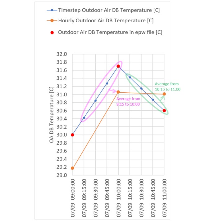
For reference, I also compared Hourly OA temperature, Timestep OA temperature and the original OA temperature in the epw file. Similarly, The Hourly OA temperature at 10:00 is the average of Timestep OA temperatures at 9:15, 9:30, 9:45 and 10:00. The Hourly OA temperatue is different from the original OA temperature in the epw file.

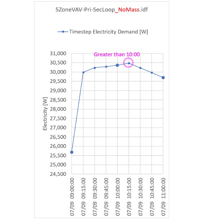
For my Question 1, I tested another case in response to @Denis Bourgeois 's comment. I changed Construction objects so that all the walls, roofs, floors and ceilings consist of Material:NoMass. Besides, WindowMaterial:Glazing and Windowmaterial:Gas were replaced to WindowMaterial:SimpleGlazingSystem. I got the following warning in the err file, but this is what I intend to do.

   ** Warning ** This building has no thermal mass which can cause an unstable solution.

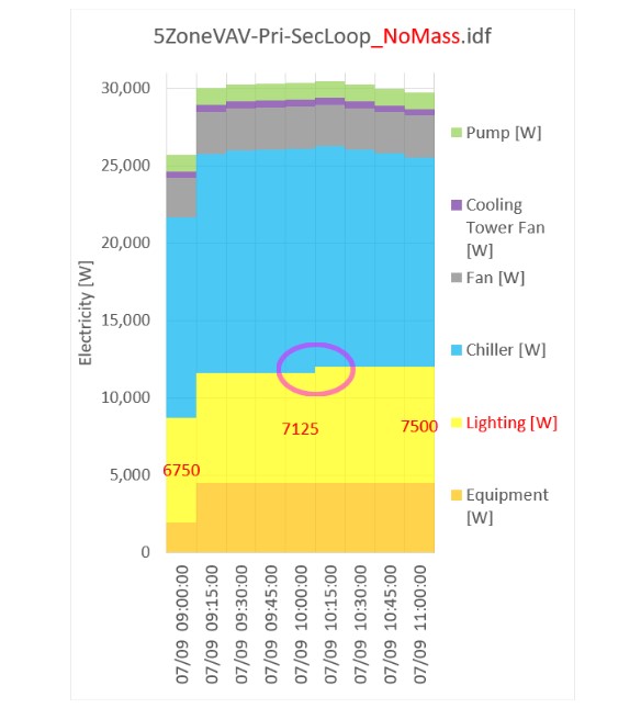
Below is the resuts of 5ZoneVAV-Pri-SecLoop_NoMass.idf. I thought the effect of delayed thermal response was removed, but the Timestep total electricity demand at 10:15 on 9 July is still higher than the demand at 10:00 on 9 July.

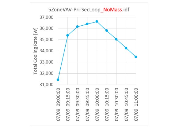
Actually, the total cooling load is the largest at 10:00 on 9 July as shown below, which makes sense.

Then, why is the total electricity demand at 10:15 larger than the total electricity demand at 10:00? The cause was simple. The lighting load was different. The chart below shows the breakdown of the total electricity demand. The lighting load of 7500W at 10:15 is larger than the lighting load of 7125W at 10:00. That's why the total electricity demand is the largest at 10:15 on 9 July.

The lighting schedule of this ExampleFile is as follows. The fraction is 0.95 at 10:00 but 1.00 at 10:15. Schedules can be modelled to be interpolated, but they are not for this ExampleFile.

Schedule:Compact,
    LIGHTS-1,                !- Name
    Fraction,                !- Schedule Type Limits Name
    Through: 12/31,          !- Field 1
    For: WeekDays SummerDesignDay CustomDay1 CustomDay2,  !- Field 2
    Until: 8:00, 0.05,       !- Field 4
    Until: 9:00, 0.9,        !- Field 6
    Until: 10:00, 0.95,      !- Field 8
    Until: 11:00, 1.00,      !- Field 10
    Until: 12:00, 0.95,      !- Field 12
    Until: 13:00, 0.8,       !- Field 14
    Until: 14:00, 0.9,       !- Field 16
    Until: 18:00, 1.00,      !- Field 18
    Until: 19:00, 0.60,      !- Field 20
    Until: 21:00, 0.40,      !- Field 22
    Until: 24:00, 0.05,      !- Field 24
    For: Weekends WinterDesignDay Holiday,  !- Field 25
    Until: 24:00, 0.05;      !- Field 27

The conclusion is that the Timestep demand can be greater than the Hourly demand depending on the combination of various factors such as weather data and schedules of people, lighting, equipment, etc.

For my Question 2, @rraustad 's comment is the answer for my Question 2. answer. The Hourly data at 10:00 is the average of Timestep data at 9:15, 9:30, 9:45 and 10:00. 10:00. I'm ashamed to say I didn't know that.

For reference, I also compared Hourly OA temperature, Timestep OA temperature and the original OA temperature in the epw file. Similarly, The Hourly OA temperature at 10:00 is the average of Timestep OA temperatures at 9:15, 9:30, 9:45 and 10:00. The Hourly OA temperatue is different from the original OA temperature in the epw file.