Question-and-Answer Resource for the Building Energy Modeling Community
| | 1 | initial version |
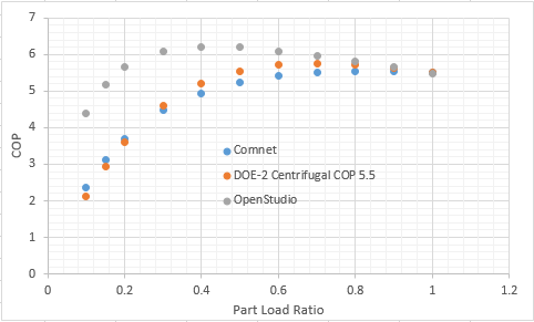
@Julien Marrec, I don't think the COPs have been calculated correctly from the given coefficients because when I take the same coefficients, calculate the COPs and plot them I get the image below.
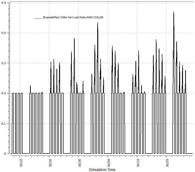
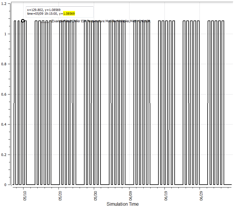
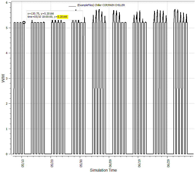
I created a test model with a chiller and used the OpenStudio curves to verify the results and viewed them in ResultsViewer. The first image is the part load ratio hourly and we'll use a reference point with a PLR of 0.2 to then look at the EIRFT and COP. At a PLR of 0.2 you I would expect a COP of 5.64 as shown in the first image above, but also at a PLR of 0.2 the EIRFT = 1.08569 and thus the actual COP for the given conditions would be 5.64/1.08 = 5.20 as can be seen in the third image below.
It looks like what you have done is calculated the EIRFPLR, but have not divided through by the PLR to get the correct EIR adjustment factor. To get the COP you first need to calculate, assuming a quadratic, the following:
EIRFPLR = a + b * PLR + c * PLR^2
The EIRFPLR value is then divided through by the PLR to get an EIR adjustment factor, which then gets multiplied by the full load EIR to get the actual EIR for a specific part load. As you know, the COP is just the inverse of this.
The variance in the curves is probably due to the type of chiller the coefficients are representing. The Comnet and DOE-2 curves looks more similar to a reciprocating chiller despite DOE-2 saying centrifugal where as the OpenStudio default looks more like a scroll chiller.
| | 2 | No.2 Revision |
@Julien Marrec, I don't think the COPs have been calculated correctly from the given coefficients because when I take the same coefficients, calculate the COPs and plot them I get the image below.
I created a test model with a chiller and used the OpenStudio curves to verify the results and viewed them in ResultsViewer. The first image is the part load ratio hourly and we'll use a reference point with a PLR of 0.2 to then look at the EIRFT and COP. At a PLR of 0.2 you I would expect a COP of 5.64 as shown in the first image above, but also at a PLR of 0.2 the EIRFT = 1.08569 and thus the actual COP for the given conditions would be 5.64/1.08 = 5.20 as can be seen in the third image below.
It looks like what you have done is calculated the EIRFPLR, but have not divided through by the PLR to get the correct EIR adjustment factor. To get the COP you first need to calculate, assuming a quadratic, the following:
EIRFPLR = a + b * PLR + c * PLR^2
The EIRFPLR value is then divided through by the PLR to get an EIR adjustment factor, which then gets multiplied by the full load EIR to get the actual EIR for a specific part load. As you know, the COP is just the inverse of this.
The variance in the curves is probably due to the type of chiller the coefficients are representing. The Comnet and DOE-2 curves looks more similar to a reciprocating chiller despite DOE-2 saying centrifugal where as the OpenStudio default looks more like a scroll chiller.
UPDATE
After reading what I wrote I realized I could make it a bit clearer. For the following segment I will use hr to denote hourly values of variables and n for the rated nominal capacity.
CAP = capacity PLR = part load ratio P = power
The capacity for a given timestep can be found as CAPhr = CAP * CAPFT and power, Phr, is expressed as:
Phr = CAPhr * EIRn * EIRFT * EIRFPLR
Assuming EIRFT is at rated conditions and thus equals 1 we get:
Phr = CAPhr * EIRn * EIRFPLR
Phr/ CAPhr = EIRn * EIRFPLR
However, we don't know CAPhr, but if we substitute in CAPhr = LOADhr/PLR then we get:
Phr * PLR / LOADhr = EIRn * EIRFPLR
Phr/LOADhr = EIRhr,
EIRhr * PLR = EIRn * EIRFPLR
Seeing as we want EIRhr we can rearrange and have all the variables known on one side and represent it as
EIRhr = EIRn * EIRFPLR / PLR
| | 3 | No.3 Revision |
@Julien Marrec, I don't think the COPs have been calculated correctly from the given coefficients because when I take the same coefficients, calculate the COPs and plot them I get the image below.
I created a test model with a chiller and used the OpenStudio curves to verify the results and viewed them in ResultsViewer. The first image is the part load ratio hourly and we'll use a reference point with a PLR of 0.2 to then look at the EIRFT and COP. At a PLR of 0.2 you I would expect a COP of 5.64 as shown in the first image above, but also at a PLR of 0.2 the EIRFT = 1.08569 and thus the actual COP for the given conditions would be 5.64/1.08 = 5.20 as can be seen in the third image below.
It looks like what you have done is calculated the EIRFPLR, but have not divided through by the PLR to get the correct EIR adjustment factor. To get the COP you first need to calculate, assuming a quadratic, the following:
EIRFPLR = a + b * PLR + c * PLR^2
The EIRFPLR value is then divided through by the PLR to get an EIR adjustment factor, which then gets multiplied by the full load EIR to get the actual EIR for a specific part load. As you know, the COP is just the inverse of this.
The variance in the curves is probably due to the type of chiller the coefficients are representing. The Comnet and DOE-2 curves looks more similar to a reciprocating chiller despite DOE-2 saying centrifugal where as the OpenStudio default looks more like a scroll chiller.
UPDATE
After reading what I wrote I realized I could make it a bit clearer. For the following segment I will use hr to denote hourly timestep values of variables and n for the rated nominal capacity.
CAP = capacity PLR = part load ratio P = power
The capacity for a given timestep can be found as CAPhr = CAP * CAPFT and power, Phr, is expressed as:
Phr = CAPhr * EIRn * EIRFT * EIRFPLR
Assuming EIRFT is at rated conditions and thus equals 1 we get:
Phr = CAPhr * EIRn * EIRFPLR
Phr/ CAPhr = EIRn * EIRFPLR
However, we don't know CAPhr, but if we substitute in CAPhr = LOADhr/PLR then we get:
Phr * PLR / LOADhr = EIRn * EIRFPLR
Phr/LOADhr = EIRhr,
EIRhr * PLR = EIRn * EIRFPLR
Seeing as we want EIRhr we can rearrange and have all the variables known on one side and represent it as
EIRhr = EIRn * EIRFPLR / PLR
| | 4 | No.4 Revision |
@Julien Marrec, I don't think the COPs have been calculated correctly from the given coefficients because when I take the same coefficients, calculate the COPs and plot them I get the image below.
I created a test model with a chiller and used the OpenStudio curves to verify the results and viewed them in ResultsViewer. The first image is the part load ratio hourly and we'll use a reference point with a PLR of 0.2 to then look at the EIRFT and COP. At a PLR of 0.2 you I would expect a COP of 5.64 as shown in the first image above, but also at a PLR of 0.2 the EIRFT = 1.08569 and thus the actual COP for the given conditions would be 5.64/1.08 = 5.20 as can be seen in the third image below.
It looks like what you have done is calculated the EIRFPLR, but have not divided through by the PLR to get the correct EIR adjustment factor. To get the COP you first need to calculate, assuming a quadratic, the following:
EIRFPLR $$EIRFPLR = a + b * \times PLR + c * PLR^2\times PLR^2$$
The EIRFPLR value is then divided through by the PLR to get an EIR adjustment factor, which then gets multiplied by the full load EIR to get the actual EIR for a specific part load. As you know, the COP is just the inverse of this.
$$EIR_{actual} = \frac{EIRFPLR \times EIR_{ref}}{PLR}$$
The variance in the curves is probably due to the type of chiller the coefficients are representing. The Comnet and DOE-2 curves looks more similar to a reciprocating chiller despite DOE-2 saying centrifugal where as the OpenStudio default looks more like a scroll chiller.
UPDATE
After reading what I wrote I realized I could make it a bit clearer. For the following segment I will use hr to denote timestep values of variables and n for the rated nominal capacity.
CAP = capacity PLR = part load ratio P = power
The capacity for a given timestep can be found as CAPhr = CAP * CAPFT and power, Phr, is expressed as:
Phr = CAPhr * EIRn * EIRFT * EIRFPLR
Assuming EIRFT is at rated conditions and thus equals 1 we get:
Phr = CAPhr * EIRn * EIRFPLR
Phr/ CAPhr = EIRn * EIRFPLR
However, we don't know CAPhr, but if we substitute in CAPhr = LOADhr/PLR then we get:
Phr * PLR / LOADhr = EIRn * EIRFPLR
Phr/LOADhr = EIRhr,
EIRhr * PLR = EIRn * EIRFPLR
Seeing as we want EIRhr we can rearrange and have all the variables known on one side and represent it as
EIRhr = EIRn * EIRFPLR / PLR
| | 5 | No.5 Revision |
@Julien Marrec, I don't think the COPs have been calculated correctly from the given coefficients because when I take the same coefficients, calculate the COPs and plot them I get the image below.
I created a test model with a chiller and used the OpenStudio curves to verify the results and viewed them in ResultsViewer. The first image is the part load ratio hourly and we'll use a reference point with a PLR of 0.2 to then look at the EIRFT and COP. At a PLR of 0.2 you I would expect a COP of 5.64 as shown in the first image above, but also at a PLR of 0.2 the EIRFT = 1.08569 and thus the actual COP for the given conditions would be 5.64/1.08 = 5.20 as can be seen in the third image below.
It looks like what you have done is calculated the EIRFPLR, but have not divided through by the PLR to get the correct EIR adjustment factor. To get the COP you first need to calculate, assuming a quadratic, the following:
$$EIRFPLR = a + b \times PLR + c \times PLR^2$$
The EIRFPLR value is then divided through by the PLR to get an EIR adjustment factor, which then gets multiplied by the full load EIR to get the actual EIR for a specific part load. As you know, the COP is just the inverse of this.
$$EIR_{actual} = \frac{EIRFPLR \times EIR_{ref}}{PLR}$$
The variance in the curves is probably due to the type of chiller the coefficients are representing. The Comnet and DOE-2 curves looks more similar to a reciprocating chiller despite DOE-2 saying centrifugal where as the OpenStudio default looks more like a scroll chiller.
UPDATE
After reading what I wrote I realized I could make it a bit clearer. For the following segment I will use hr $hr$ to denote timestep values of variables and n $n$ for the rated nominal capacity.
CAP = capacity PLR
The capacity for a given timestep can be found as CAPhr $CAP_{hr} = CAP * CAPFT \times CAPFT$ and power, Phr, $P_{hr}$, is expressed as:
Phr = CAPhr * EIRn * $$P_{hr} = CAP_{hr} \times EIR_{n} \times EIRFT * EIRFPLR\times EIRFPLR$$
Assuming EIRFT $EIRFT$ is at rated conditions and thus equals 1 we get:
Phr = CAPhr * EIRn * EIRFPLR
Phr/ CAPhr = EIRn * EIRFPLR$$P_{hr} = CAP_{hr} \times EIR_{n} \times EIRFPLR$$
$$\frac{P_{hr}}{CAP_{hr}} = EIR_{n} \times EIRFPLR$$
However, we don't know CAPhr, $CAP_{hr}$, but if we substitute in CAPhr = LOADhr/PLR $CAP_{hr} = \frac{LOAD_{hr}}{PLR}$ then we get:
Phr * PLR / LOADhr = EIRn * EIRFPLR
Phr/LOADhr = EIRhr,
EIRhr * PLR = EIRn * EIRFPLR$$P_{hr} \times \frac{PLR}{LOAD_{hr}} = EIR_{n} \times EIRFPLR$$
$$\frac{P_{hr}}{LOAD_{hr}} = EIR_{hr}$$
$$EIR_{hr} \times PLR = EIR_{n} \times EIRFPLR$$
Seeing as we want EIRhr $EIR_{hr}$ we can rearrange and have all the variables known on one side and represent it as
EIRhr = EIRn * EIRFPLR / PLR


