Question-and-Answer Resource for the Building Energy Modeling Community
Get started with the Help page
Ask Your Question

Revision history [back]

click to hide/show revision 1
initial version

Constant vs. nighttime-reduced temperature

Hello,

As a new Open Studio user, I conducted a bunch of simulations to understand the impact of different parameters. Among these simulations, a case bothers me.

(Sorry, but as a new user I cannot post pictures... I had to insert links to files)

The basic version consists of a simple cube (no windows, no internal gains, no infiltration, no ventilation ...). The temperature is set to 22 °C (constant) and I make use of the "ideal air loads system". The results seem consistent (see green values in the file, which are also found in the graph)

Results without nighttime-reduced temperature

Graphic

The second version is identical but incorporating a temperature reduction at night and on weekends (16°C instead of 22°C). Of course I understand that some heating-up capacity is necessary, but this does not explain all the results.

Results with nighttime-reduced temperature

Graphic

  1. "calculated design load" is identical in both cases, which makes sense
  2. in the basic version, "district heating" is 3137.46W and corresponds to the peak on the graph : OK
  3. in the modified version, "district heating" is 23513.39W (almost 8 x higher). This value does not match the peak on the graph (about 9750 W). Is there an explanation?
  4. in "energy meters", why is "Energy Transfer Partners: Facility" (20183.82 W) slightly different than "DistrictHeating:Facility" (23513.39 W) ?
  5. where does "HVAC area eq. & Other sensitive air heating" value (188925.97 W) come from ?

Could you help me? Am I missing something?

I understand that this is an "extreme" case, and that in reality the differences will be smaller thanks to internal and solar gains (I tried a real case, and there is an order of magnitude of +/- 2).

Without modeling a complete HVAC system, is there a way to get closer to a real heating system (with limited capacity)?

Thank you very much for your time.

Nicolas

Constant vs. nighttime-reduced temperatureSizing vs simulation peak power difference

Hello,

As a new Open Studio user, I conducted a bunch of simulations to understand the impact of different parameters. Among these simulations, a case bothers me.

(Sorry, but as a new user I cannot post pictures... I had to insert links to files)

The basic version consists of a simple cube (no windows, no internal gains, no infiltration, no ventilation ...). The temperature is set to 22 °C (constant) and I make use of the "ideal air loads system". The results seem consistent (see green values in the file, which are also found in the graph)

Results without nighttime-reduced temperature

Graphic

The second version is identical but incorporating a temperature reduction at night and on weekends (16°C instead of 22°C). Of course I understand that some heating-up capacity is necessary, but this does not explain all the results.

Results with nighttime-reduced temperature

Graphic

  1. "calculated design load" is identical in both cases, which makes sense
  2. in the basic version, "district heating" is 3137.46W and corresponds to the peak on the graph : OK
  3. in the modified version, "district heating" is 23513.39W (almost 8 x higher). This value does not match the peak on the graph (about 9750 W). Is there an explanation?
  4. in "energy meters", why is "Energy Transfer Partners: Facility" (20183.82 W) slightly different than "DistrictHeating:Facility" (23513.39 W) ?
  5. where does "HVAC area eq. & Other sensitive air heating" value (188925.97 W) come from ?

Could you help me? Am I missing something?

I understand that this is an "extreme" case, and that in reality the differences will be smaller thanks to internal and solar gains (I tried a real case, and there is an order of magnitude of +/- 2).

Without modeling a complete HVAC system, is there a way to get closer to a real heating system (with limited capacity)?

Thank you very much for your time.

Nicolas

EDIT

From what I could see, the use of "Timesteps in Averaging Window" only affects the "design load" value in the report. This will certainly help me in other situations, but in fact, my question is not really about sizing (I used constant temperature set point) but the complete runperiod.

I could finally find some values ​​by performing the simulation on a day (thank you for the tip), but there are certain factors that I can not explain :

image description

  • 1.176 coefficient between "EnergyTransfer:Facility" and "DistrictHeating:Facility"
  • 1.336 coefficient between the peak on the graph and the "design load" value
  • 10 coefficient between the peak on the graph and the "peak heating sensible heat gain" value

If I use a constant schedule, these three factors are exactly 1 ...

Currently, I use "ideal loads air system". I would have to take the time to create a measure which limits the power to the "design load" value calculated in a previous run...

Here is a link to the idf file if it can help you :

IDF file

Thanks

Sizing vs simulation peak power difference

Hello,

As a new Open Studio user, I conducted a bunch of simulations to understand the impact of different parameters. Among these simulations, a case bothers me.

(Sorry, but as a new user I cannot post pictures... I had to insert links to files)

The basic version consists of a simple cube (no windows, no internal gains, no infiltration, no ventilation ...). The temperature is set to 22 °C (constant) and I make use of the "ideal air loads system". The results seem consistent (see green values in the file, which are also found in the graph)

Results without nighttime-reduced temperature

Graphic

The second version is identical but incorporating a temperature reduction at night and on weekends (16°C instead of 22°C). Of course I understand that some heating-up capacity is necessary, but this does not explain all the results.

Results with nighttime-reduced temperature

Graphic

  1. "calculated design load" is identical in both cases, which makes sense
  2. in the basic version, "district heating" is 3137.46W and corresponds to the peak on the graph : OK
  3. in the modified version, "district heating" is 23513.39W (almost 8 x higher). This value does not match the peak on the graph (about 9750 W). Is there an explanation?
  4. in "energy meters", why is "Energy Transfer Partners: Facility" (20183.82 W) slightly different than "DistrictHeating:Facility" (23513.39 W) ?
  5. where does "HVAC area eq. & Other sensitive air heating" value (188925.97 W) come from ?

Could you help me? Am I missing something?

I understand that this is an "extreme" case, and that in reality the differences will be smaller thanks to internal and solar gains (I tried a real case, and there is an order of magnitude of +/- 2).

Without modeling a complete HVAC system, is there a way to get closer to a real heating system (with limited capacity)?

Thank you very much for your time.

Nicolas
EDIT

From what I could see, the use of "Timesteps in Averaging Window" only affects the "design load" value in the report. This will certainly help me in other situations, but in fact, my question is not really about sizing (I used constant temperature set point) but the complete runperiod.

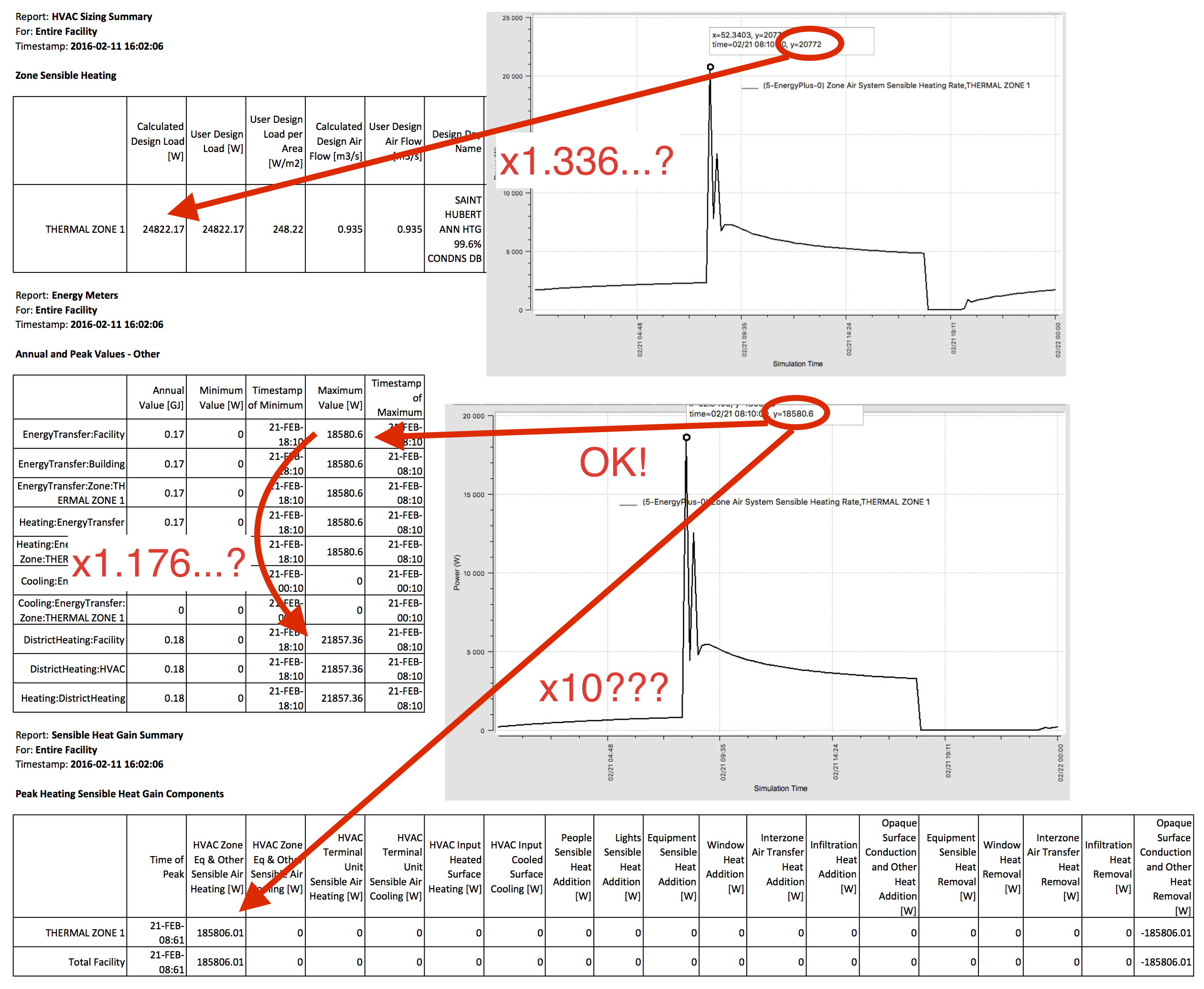
I could finally find some values ​​by performing the simulation on a day (thank you for the tip), but there are certain factors that I can not explain :

image description

  • 1.176 coefficient between "EnergyTransfer:Facility" and "DistrictHeating:Facility"
  • 1.336 coefficient between the peak on the graph and the "design load" value
  • 10 coefficient between the peak on the graph and the "peak heating sensible heat gain" value

If I use a constant schedule, these three factors are exactly 1 ...

Currently, I use "ideal loads air system". I would have to take the time to create a measure which limits the power to the "design load" value calculated in a previous run...

Here is a link to the idf file if it can help you :

IDF file

Thanks

Sizing vs simulation peak power difference

Hello,

As a new Open Studio user, I conducted a bunch of simulations to understand the impact of different parameters. Among these simulations, a case bothers me.

(Sorry, but as a new user I cannot post pictures... I had to insert links to files)

The basic version consists of a simple cube (no windows, no internal gains, no infiltration, no ventilation ...). The temperature is set to 22 °C (constant) and I make use of the "ideal air loads system". The results seem consistent (see green values in the file, which are also found in the graph)

Results without nighttime-reduced temperature

Graphic

The second version is identical but incorporating a temperature reduction at night and on weekends (16°C instead of 22°C). Of course I understand that some heating-up capacity is necessary, but this does not explain all the results.

Results with nighttime-reduced temperature

Graphic

  1. "calculated design load" is identical in both cases, which makes sense
  2. in the basic version, "district heating" is 3137.46W and corresponds to the peak on the graph : OK
  3. in the modified version, "district heating" is 23513.39W (almost 8 x higher). This value does not match the peak on the graph (about 9750 W). Is there an explanation?
  4. in "energy meters", why is "Energy Transfer Partners: Facility" (20183.82 W) slightly different than "DistrictHeating:Facility" (23513.39 W) ?
  5. where does "HVAC area eq. & Other sensitive air heating" value (188925.97 W) come from ?

Could you help me? Am I missing something?

I understand that this is an "extreme" case, and that in reality the differences will be smaller thanks to internal and solar gains (I tried a real case, and there is an order of magnitude of +/- 2).

Without modeling a complete HVAC system, is there a way to get closer to a real heating system (with limited capacity)?

Thank you very much for your time.

Nicolas

EDIT

From what I could see, the use of "Timesteps in Averaging Window" only affects the "design load" value in the report. This will certainly help me in other situations, but in fact, my question is not really about sizing (I used constant temperature set point) but the complete runperiod.

I could finally find some values ​​by performing the simulation on a day (thank you for the tip), but there are certain factors that I can not explain :

image description

  • 1.176 coefficient between "EnergyTransfer:Facility" and "DistrictHeating:Facility"
  • 1.336 coefficient between the peak on the graph and the "design load" value
  • 10 coefficient between the peak on the graph and the "peak heating sensible heat gain" value

If I use a constant schedule, these three factors are exactly 1 ...

Currently, I use "ideal loads air system". I would have to take the time to create a measure which limits the power to the "design load" value calculated in a previous run...

Here is a link to the idf file if it can help you :

IDF file

Thanks

Sizing vs simulation peak power difference

Hello,

As a new Open Studio user, I conducted a bunch of simulations to understand the impact of different parameters. Among these simulations, a case bothers me.

(Sorry, but as a new user I cannot post pictures... I had to insert links to files)

The basic version consists of a simple cube (no windows, no internal gains, no infiltration, no ventilation ...). The temperature is set to 22 °C (constant) and I make use of the "ideal air loads system". The results seem consistent (see green values in the file, which are also found in the graph)

Results without nighttime-reduced temperature

Graphic

The second version is identical but incorporating a temperature reduction at night and on weekends (16°C instead of 22°C). Of course I understand that some heating-up capacity is necessary, but this does not explain all the results.

Results with nighttime-reduced temperature

Graphic

  1. "calculated design load" is identical in both cases, which makes sense
  2. in the basic version, "district heating" is 3137.46W and corresponds to the peak on the graph : OK
  3. in the modified version, "district heating" is 23513.39W (almost 8 x higher). This value does not match the peak on the graph (about 9750 W). Is there an explanation?
  4. in "energy meters", why is "Energy Transfer Partners: Facility" (20183.82 W) slightly different than "DistrictHeating:Facility" (23513.39 W) ?
  5. where does "HVAC area eq. & Other sensitive air heating" value (188925.97 W) come from ?

Could you help me? Am I missing something?

I understand that this is an "extreme" case, and that in reality the differences will be smaller thanks to internal and solar gains (I tried a real case, and there is an order of magnitude of +/- 2).

Without modeling a complete HVAC system, is there a way to get closer to a real heating system (with limited capacity)?

Thank you very much for your time.

Nicolas

EDIT

From what I could see, the use of "Timesteps in Averaging Window" only affects the "design load" value in the report. This will certainly help me in other situations, but in fact, my question is not really about sizing (I used constant temperature set point) but the complete runperiod.

I could finally find some values ​​by performing the simulation on a day (thank you for the tip), but there are certain factors that I can not explain :

image description

  • 1.176 coefficient between "EnergyTransfer:Facility" and "DistrictHeating:Facility"
  • 1.336 coefficient between the peak on the graph and the "design load" value
  • 10 coefficient between the peak on the graph and the "peak heating sensible heat gain" value

If I use a constant schedule, these three factors are exactly 1 ...

Currently, I use "ideal loads air system". I would have to take the time to create a measure which limits the power to the "design load" value calculated in a previous run...

Here is a link to the idf file if it can help you :

IDF file

Thanks