First time here? Check out the Help page!
 | 1 | initial version |
Since you mention Leaving water temperature, I assume you are using Chiller:Electric:ReformulatedEIR. There are 3 curves, Cooling Capacity Function of Temperature Curve Name and Electric Input to Cooling Output Ratio Function of Temperature Curve Name are both a function of leaving chilled and condenser fluid temperatures. Your 2nd table shows this data. The final curve is Electric Input to Cooling Output Ratio Function of Part Load Ratio Curve Name which is a function of part-load ratio. I think you meant to create this curve using your first table. However, I see what looks like a flow rate instead of part-load ratio which would be numbers between 0 and 1. You should also plot your curves using a spreadsheet. For example plot Cooling Capacity Function of Temperature Curve result versus leaving condenser water temperature for discrete leaving chilled water temperatures (plot data only for 7C, then other data for 9 C, etc.). This way you can see how the curve behaves at different temperatures. Also do this for the Electric Input to Cooling Output Ratio Function of Temperature Curve.
 | 2 | No.2 Revision |
Since you mention Leaving water temperature, I assume you are using Chiller:Electric:ReformulatedEIR. There are 3 curves, Cooling Capacity Function of Temperature Curve Name and Electric Input to Cooling Output Ratio Function of Temperature Curve Name are both a function of leaving chilled and condenser fluid temperatures. Your 2nd table shows this data. The final curve is Electric Input to Cooling Output Ratio Function of Part Load Ratio Curve Name which is a function of part-load ratio. I think you meant to create this curve using your first table. However, I see what looks like a flow rate instead of part-load ratio which would be numbers between 0 and 1. You should also plot your curves using a spreadsheet. For example plot Cooling Capacity Function of Temperature Curve result versus leaving condenser water temperature for discrete leaving chilled water temperatures (plot data only for 7C, then other data for 9 C, etc.). This way you can see how the curve behaves at different temperatures. Also do this for the Electric Input to Cooling Output Ratio Function of Temperature Curve.
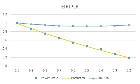
I plotted your EIRfPLR curve and it doesn't look right. This curve should go to 0 as PLR goes to 0. This means you are getting full power at low part-load conditions and would explain the low COP numbers. The EIRFPLR curve is really a power ratio curve. Compare the power ratio at each PLR or at PLR = 0.2 then the power ratio is
Power ratio = 28.97 kw / 153.8 kW = 0.18836. Creating regression coefficient in Excel is easy once you know how to do it. The document I provided shows exactly how to do that and I'm sure you can find lots of information on the web.
Your curve coefficients:
Curve:Quadratic,
  ChlrAirScrollEIRRatio_fQRatio,          !- Name
  1.0069198702,                           !- Coefficient1 Constant
  -0.3099076705,                          !- Coefficient2 x
  0.3029878003,                           !- Coefficient3 x**2
My curve coefficients:
Curve:Quadratic,
  ChlrAirScrollEIRRatio_fQRatio,          !- Name
  0.053494024,                            !- Coefficient1 Constant
  0.672923035,                            !- Coefficient2 x
  0.266558864,                            !- Coefficient3 x**2
 | 3 | No.3 Revision |
Since you mention Leaving water temperature, I assume you are using Chiller:Electric:ReformulatedEIR. There are 3 curves, Cooling Capacity Function of Temperature Curve Name and Electric Input to Cooling Output Ratio Function of Temperature Curve Name are both a function of leaving chilled and condenser fluid temperatures. Your 2nd table shows this data. The final curve is Electric Input to Cooling Output Ratio Function of Part Load Ratio Curve Name which is a function of part-load ratio. I think you meant to create this curve using your first table. However, I see what looks like a flow rate instead of part-load ratio which would be numbers between 0 and 1. You should also plot your curves using a spreadsheet. For example plot Cooling Capacity Function of Temperature Curve result versus leaving condenser water temperature for discrete leaving chilled water temperatures (plot data only for 7C, then other data for 9 C, etc.). This way you can see how the curve behaves at different temperatures. Also do this for the Electric Input to Cooling Output Ratio Function of Temperature Curve.
I plotted your EIRfPLR curve and it doesn't look right. This curve should go to 0 as PLR goes to 0. This means you are getting full power at low part-load conditions and would explain the low COP numbers. The EIRFPLR curve is really a power ratio curve. Compare the power ratio at each PLR or at PLR = 0.2 then the power ratio is
Power ratio = 28.97 kw / 153.8 kW = 0.18836. Creating regression coefficient in Excel is easy once you know how to do it. The document I provided shows exactly how to do that and I'm sure you can find lots of information on the web.
Your curve coefficients:
Curve:Quadratic,
  ChlrAirScrollEIRRatio_fQRatio,          !- Name
  1.0069198702,                           !- Coefficient1 Constant
  -0.3099076705,                          !- Coefficient2 x
  0.3029878003,                           !- Coefficient3 x**2
My curve coefficients:
Curve:Quadratic,
  ChlrAirScrollEIRRatio_fQRatio,          !- Name
  0.053494024,                            !- Coefficient1 Constant
  0.672923035,                            !- Coefficient2 x
  0.266558864,                            !- Coefficient3 x**2
 | 4 | No.4 Revision |
Since you mention Leaving water temperature, I assume you are using Chiller:Electric:ReformulatedEIR. There are 3 curves, Cooling Capacity Function of Temperature Curve Name and Electric Input to Cooling Output Ratio Function of Temperature Curve Name are both a function of leaving chilled and condenser fluid temperatures. Your 2nd table shows this data. The final curve is Electric Input to Cooling Output Ratio Function of Part Load Ratio Curve Name which is a function of part-load ratio. I think you meant to create this curve using your first table. However, I see what looks like a flow rate instead of part-load ratio which would be numbers between 0 and 1. You should also plot your curves using a spreadsheet. For example plot Cooling Capacity Function of Temperature Curve result versus leaving condenser water temperature for discrete leaving chilled water temperatures (plot data only for 7C, then other data for 9 C, etc.). This way you can see how the curve behaves at different temperatures. Also do this for the Electric Input to Cooling Output Ratio Function of Temperature Curve.
I plotted your EIRfPLR curve and it doesn't look right. This curve should go to 0 as PLR goes to 0. This means you are getting full power at low part-load conditions and would explain the low COP numbers. The EIRFPLR curve is really a power ratio curve. Compare the power ratio at each PLR or at PLR = 0.2 then the power ratio is
Power ratio = 28.97 kw / 153.8 kW = 0.18836.
Creating regression coefficient in Excel is easy once you know how to do it. The document I provided shows exactly how to do that and I'm sure you can find lots of information on the web.
Your curve coefficients:
Curve:Quadratic,
  ChlrAirScrollEIRRatio_fQRatio,          !- Name
  1.0069198702,                           !- Coefficient1 Constant
  -0.3099076705,                          !- Coefficient2 x
  0.3029878003,                           !- Coefficient3 x**2
My curve coefficients:
Curve:Quadratic,
  ChlrAirScrollEIRRatio_fQRatio,          !- Name
  0.053494024,                            !- Coefficient1 Constant
  0.672923035,                            !- Coefficient2 x
  0.266558864,                            !- Coefficient3 x**2
 | 5 | No.5 Revision |
Since you mention Leaving water temperature, I assume you are using Chiller:Electric:ReformulatedEIR. There are 3 curves, Cooling Capacity Function of Temperature Curve Name and Electric Input to Cooling Output Ratio Function of Temperature Curve Name are both a function of leaving chilled and condenser fluid temperatures. Your 2nd table shows this data. The final curve is Electric Input to Cooling Output Ratio Function of Part Load Ratio Curve Name which is a function of part-load ratio. I think you meant to create this curve using your first table. However, I see what looks like a flow rate instead of part-load ratio which would be numbers between 0 and 1. You should also plot your curves using a spreadsheet. For example plot Cooling Capacity Function of Temperature Curve result versus leaving condenser water temperature for discrete leaving chilled water temperatures (plot data only for 7C, then other data for 9 C, etc.). This way you can see how the curve behaves at different temperatures. Also do this for the Electric Input to Cooling Output Ratio Function of Temperature Curve.
I plotted your EIRfPLR curve and it doesn't look right. This curve should go to 0 as PLR goes to 0. This means you are getting full power at low part-load conditions and would explain the low COP numbers. The EIRFPLR curve is really a power ratio curve. Compare the power ratio at each PLR or at PLR = 0.2 then the power ratio is
Power ratio = 28.97 kw / 153.8 kW = 0.18836.
Creating regression coefficient in Excel is easy once you know how to do it. The document I provided shows exactly how to do that and I'm sure you can find lots of information on the web.
Your curve coefficients:
Curve:Quadratic,
  ChlrAirScrollEIRRatio_fQRatio,          !- Name
  1.0069198702,                           !- Coefficient1 Constant
  -0.3099076705,                          !- Coefficient2 x
  0.3029878003,                           !- Coefficient3 x**2
My curve coefficients:
Curve:Quadratic,
  ChlrAirScrollEIRRatio_fQRatio,          !- Name
  0.053494024,                            !- Coefficient1 Constant
  0.672923035,                            !- Coefficient2 x
  0.266558864,                            !- Coefficient3 x**2

Here is the power equation directly from the code.
Power = (AvailChillerCap / ReferenceCOP) * ChillerEIRFPLR * ChillerEIRFT * FRAC;
where: AvailChillerCap is the full load output at current operating condition of Tevapin and Tout ReferenceCOP is the rated COP ChillerEIRfPLR is the curve discussed here ChillerEIRFT is the EIR as a function of temperatures and FRAC is when the chiller cycles below min PLR, above min PLR then FRAC = 1
 | 6 | No.6 Revision |
Since you mention Leaving water temperature, I assume you are using Chiller:Electric:ReformulatedEIR. There are 3 curves, Cooling Capacity Function of Temperature Curve Name and Electric Input to Cooling Output Ratio Function of Temperature Curve Name are both a function of leaving chilled and condenser fluid temperatures. Your 2nd table shows this data. The final curve is Electric Input to Cooling Output Ratio Function of Part Load Ratio Curve Name which is a function of part-load ratio. I think you meant to create this curve using your first table. However, I see what looks like a flow rate instead of part-load ratio which would be numbers between 0 and 1. You should also plot your curves using a spreadsheet. For example plot Cooling Capacity Function of Temperature Curve result versus leaving condenser water temperature for discrete leaving chilled water temperatures (plot data only for 7C, then other data for 9 C, etc.). This way you can see how the curve behaves at different temperatures. Also do this for the Electric Input to Cooling Output Ratio Function of Temperature Curve.
I plotted your EIRfPLR curve and it doesn't look right. This curve should go to 0 as PLR goes to 0. This means you are getting full power at low part-load conditions and would explain the low COP numbers. The EIRFPLR curve is really a power ratio curve. Compare the power ratio at each PLR or at PLR = 0.2 then the power ratio is
Power ratio = 28.97 kw / 153.8 kW = 0.18836.
Creating regression coefficient in Excel is easy once you know how to do it. The document I provided shows exactly how to do that and I'm sure you can find lots of information on the web.
Your curve coefficients:
Curve:Quadratic,
  ChlrAirScrollEIRRatio_fQRatio,          !- Name
  1.0069198702,                           !- Coefficient1 Constant
  -0.3099076705,                          !- Coefficient2 x
  0.3029878003,                           !- Coefficient3 x**2
My curve coefficients:
Curve:Quadratic,
  ChlrAirScrollEIRRatio_fQRatio,          !- Name
  0.053494024,                            !- Coefficient1 Constant
  0.672923035,                            !- Coefficient2 x
  0.266558864,                            !- Coefficient3 x**2

Here is the power equation directly from the code.
Power = (AvailChillerCap / ReferenceCOP) * ChillerEIRFPLR * ChillerEIRFT * FRAC;
where:
where:
AvailChillerCap is the full load output at current operating condition of Tevapin and Tout
Tout
ReferenceCOP is the rated COP
COP
ChillerEIRfPLR is the curve discussed here
here
ChillerEIRFT is the EIR as a function of temperatures
temperatures
and FRAC is when the chiller cycles below min PLR, above min PLR then FRAC = 1
 | 7 | No.7 Revision |
Since you mention Leaving water temperature, I assume you are using Chiller:Electric:ReformulatedEIR. There are 3 curves, Cooling Capacity Function of Temperature Curve Name and Electric Input to Cooling Output Ratio Function of Temperature Curve Name are both a function of leaving chilled and condenser fluid temperatures. Your 2nd table shows this data. The final curve is Electric Input to Cooling Output Ratio Function of Part Load Ratio Curve Name which is a function of part-load ratio. I think you meant to create this curve using your first table. However, I see what looks like a flow rate instead of part-load ratio which would be numbers between 0 and 1. You should also plot your curves using a spreadsheet. For example plot Cooling Capacity Function of Temperature Curve result versus leaving condenser water temperature for discrete leaving chilled water temperatures (plot data only for 7C, then other data for 9 C, etc.). This way you can see how the curve behaves at different temperatures. Also do this for the Electric Input to Cooling Output Ratio Function of Temperature Curve.
I plotted your EIRfPLR curve and it doesn't look right. This curve should go to 0 as PLR goes to 0. This means you are getting full power at low part-load conditions and would explain the low COP numbers. The EIRFPLR curve is really a power ratio curve. Compare the power ratio at each PLR or if power is 28.97 kW at PLR = 0.1 and power is 153.8 kW at PLR = 1 then at PLR = 0.2 then the power ratio is
Power ratio = 28.97 kw / 153.8 kW = 0.18836.
Creating regression coefficient in Excel is easy once you know how to do it. The document I provided shows exactly how to do that and I'm sure you can find lots of information on the web.
Your curve coefficients:
Curve:Quadratic,
  ChlrAirScrollEIRRatio_fQRatio,          !- Name
  1.0069198702,                           !- Coefficient1 Constant
  -0.3099076705,                          !- Coefficient2 x
  0.3029878003,                           !- Coefficient3 x**2
My curve coefficients:
Curve:Quadratic,
  ChlrAirScrollEIRRatio_fQRatio,          !- Name
  0.053494024,                            !- Coefficient1 Constant
  0.672923035,                            !- Coefficient2 x
  0.266558864,                            !- Coefficient3 x**2

Here is the power equation directly from the code.
Power = (AvailChillerCap / ReferenceCOP) * ChillerEIRFPLR * ChillerEIRFT * FRAC;
where:
AvailChillerCap is the full load output at current operating condition of Tevapin and Tout
ReferenceCOP is the rated COP
ChillerEIRfPLR is the curve discussed here
ChillerEIRFT is the EIR as a function of temperatures
and FRAC is when the chiller cycles below min PLR, above min PLR then FRAC = 1
 | 8 | No.8 Revision |
Since you mention Leaving water temperature, I assume you are using Chiller:Electric:ReformulatedEIR. There are 3 curves, Cooling Capacity Function of Temperature Curve Name and Electric Input to Cooling Output Ratio Function of Temperature Curve Name are both a function of leaving chilled and condenser fluid temperatures. Your 2nd table shows this data. The final curve is Electric Input to Cooling Output Ratio Function of Part Load Ratio Curve Name which is a function of part-load ratio. I think you meant to create this curve using your first table. However, I see what looks like a flow rate instead of part-load ratio which would be numbers between 0 and 1. You should also plot your curves using a spreadsheet. For example plot Cooling Capacity Function of Temperature Curve result versus leaving condenser water temperature for discrete leaving chilled water temperatures (plot data only for 7C, then other data for 9 C, etc.). This way you can see how the curve behaves at different temperatures. Also do this for the Electric Input to Cooling Output Ratio Function of Temperature Curve.
I plotted your EIRfPLR curve and it doesn't look right. This curve should go to 0 as PLR goes to 0. This means you are getting full power at low part-load conditions and would explain the low COP numbers. The EIRFPLR curve is really a power ratio curve. Compare the power ratio at each PLR or if power is 28.97 kW at PLR = 0.1 0.2 and power is 153.8 kW at PLR = 1 then at PLR = 0.2 then the power ratio is
Power ratio = 28.97 kw / 153.8 kW = 0.18836.
Creating regression coefficient in Excel is easy once you know how to do it. The document I provided shows exactly how to do that and I'm sure you can find lots of information on the web.
Your curve coefficients:
Curve:Quadratic,
  ChlrAirScrollEIRRatio_fQRatio,          !- Name
  1.0069198702,                           !- Coefficient1 Constant
  -0.3099076705,                          !- Coefficient2 x
  0.3029878003,                           !- Coefficient3 x**2
My curve coefficients:
Curve:Quadratic,
  ChlrAirScrollEIRRatio_fQRatio,          !- Name
  0.053494024,                            !- Coefficient1 Constant
  0.672923035,                            !- Coefficient2 x
  0.266558864,                            !- Coefficient3 x**2

Here is the power equation directly from the code.
Power = (AvailChillerCap / ReferenceCOP) * ChillerEIRFPLR * ChillerEIRFT * FRAC;
where:
AvailChillerCap is the full load output at current operating condition of Tevapin and Tout
ReferenceCOP is the rated COP
ChillerEIRfPLR is the curve discussed here
ChillerEIRFT is the EIR as a function of temperatures
and FRAC is when the chiller cycles below min PLR, above min PLR then FRAC = 1
